Tensor Networks
Linear response in quantum chemistry
The particle-hole random phase approximation in density functional theory
The random phase approximation of TDDFT
Anderson acceleration
Solid state physics

Research interests

My research work focuses on the numerical and theoretical analysis of numerical models and methods in quantum chemistry, whether they come from solid state physics or molecular chemistry. More precisely, they aim to estimate the errors that have several possible origins

modeling errors: the equations which govern quantum chemistry are known - the Schrödinger equation is a high-dimensional linear PDE - which can only be solved for systems reduced to a few electrons. The models (Hartree-Fock or Kohn-Sham) reduce the problem to solving a nonlinear system of PDEs in 3D.
discretization errors: for a given model, this error depends on the numerical scheme considered (plane waves, finite elements or finite differences).
algorithmic errors: at a fixed model and scheme, the chosen algorithm introduces an error which may be difficult to assess. The nonlinear PDEs in quantum chemistry are solved by fixed point methods. The underlying problem being in the vast majority of cases non-convex, the convergence with respect to a numerical tolerance is unclear.

Tensor Networks

Tensor Networks (TN) have seen rapid and emerging interests. They aim to give a sparse representation of high-dimensional functions. The first instance of TN was Matrix Product States (MPS) or Tensor Trains that were introduced in the late 90s/early 2000s in physics as DMRG (Density Matrix Renormalization Group) to find the ground-state of statistical models (one-dimensional Hubbard or Heisenberg models). MPS has been used for the $N$ -body electronic Schrödinger problem where the question of the optimal topology (or best ordering) is not clear.

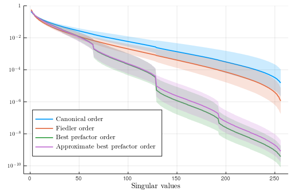
In the contribution, we investigate the behaviour of the singular values of reshapes of a particular class of functions (Slater determinants). The decay of these singular values drives the approximability of the function by an MPS. For this class of functions, if we denote by $(\sigma_j)$ the singular values of the reshaped tensor $\Psi_{\mu_1 \dots \mu_{L/2}}^{\mu_{L/2+1}\dots \mu_L}$ , then we show that there are $2^N$ positive singular values, where $N$ is the number of particles and they satisfy

\sigma_1 \sigma_{2^N} = \sigma_2 \sigma_{2^N-1} = \sigma_3 \sigma_{2^N-2} = \cdots = \mathrm{Const}.

The constant is moreover explicit and depends on the ordering of the modes of the tensor. This provides a natural criterion to optimze a TT approximation of the state.

Singular values of the reshaped tensor for different ordering schemes

Publication

Mi-Song Dupuy, Gero Friesecke, Inversion symmetry of singular values and a new orbital ordering method in tensor train approximations for quantum chemistry, SIAM Journal on Scientific Computing, 2021.

Linear response in quantum chemistry

Properties of a molecule in its ground-state perturbed by a time-dependent potential can be approximated in the linear regime (assuming that the perturbation is small) using the Kubo formula. To be more precise, if $\psi_0$ is the ground-state of $H = -\Delta + V$ an operator acting on $L^2(\mathbb{R}^d)$ , for some observable $V_\mathcal{O}$ and $\psi(t)$ solution to

i\partial_{t} \psi = H \psi + \varepsilon f(t) V_{\mathcal P} \psi , \quad \psi(0) = \psi_{0},

the linear response function $K$ defined by

\langle \psi(t), V_{\mathcal O} \psi(t) \rangle = \Big\langle \psi_{0}, V_{\mathcal O} \psi_{0}\Big\rangle + \varepsilon (K \ast f)(t) + \mathcal{O}(\varepsilon^2),

is given by the Kubo formula

K(\tau) = -i \theta(\tau) \Big\langle V_{\mathcal O} \psi_{0}, e^{-i (H-E_{0}) \tau} V_{\mathcal P} \psi_{0}\Big\rangle + {\rm c.c.}.

The Fourier transform of $K$ is then

\widehat K(\omega) = \lim_{\eta \to 0^{+}} \Big\langle \psi_{0}, V_{\mathcal O} \Big(\omega +i\eta - (H-E_0)\Big)^{-1} V_{\mathcal P} \psi_{0}\Big\rangle - \Big\langle \psi_{0},V_{\mathcal P} \Big(\omega +i\eta + (H-E_0)\Big)^{-1} V_{\mathcal O} \psi_{0}\Big\rangle.

The above formula is in practice approximated by taking a positive $\eta$ and by truncating the space to a finite region $(-L,L)^d$ . This necessarily yields a singular approximation of the linear response function $\widehat{K}$ . In the paper, the regularity of the response function $\widehat{K}$ is determined, depending on the decay of the potential $V$ . Moreover, the relationship between $\eta$ and $L$ guaranteeing the convergence of the approximation is shown, supported by numerical experiments.

Publication

Mi-Song Dupuy, Antoine Levitt, Finite-size effects in response functions of molecular systems, accepted in SMAI Journal of Computational Mathematics, 2022.

The particle-hole random phase approximation in density functional theory

The ground-state of a molecule is given by the lowest eigenvalue of the operator $H_N$ acting on $\bigwedge_{i=1}^N L^2(\mathbb{R}^3\times \mathbb{Z}_2)$ with domain $H^2(\mathbb{R}^{3N}\times \mathbb{Z}_2)$

H_N(v_\mathrm{ext},w) = \sum\limits_{i=1}^N \Big(-\frac{1}{2}\Delta_{r_i} + v_{\mathrm{ext}}(r_i) \Big) + \sum\limits_{1 \leq i < j \leq N} w(r_i-r_j),

where $N$ is the number of electrons, $v_\mathrm{ext}$ accounts for the interaction with the nuclei and $w$ is the electron-electron interaction. Solving the high-dimensional eigenvalue problem is quickly intractable for systems with more than a few electrons, but thankfully, the ground state energy can be computed using density functional theory (DFT). DFT states the existence of a universal functional $F$ of the electronic density $\rho(r) = N\int_{\mathbb{R}^{3(N-1)}} |\Psi_0(r,\overline{r})|^2 \, \mathrm{d}\overline{r}$ such that

E_0 = \min_{\|\Psi\|=1} \langle \Psi, H_N \Psi \rangle = \min_{\rho \in \mathcal{I}_N} F(\rho) + \langle v_{\mathrm{ext}}, \rho\rangle,

where $\mathcal{I}_N$ is the admissible set of electronic densities.

It is a tremendous reduction of dimensionality, at the expense that the functional $F$ is unknown... Over the past 60 years, great efforts have been put in the design of more and more accurate density functionals, that have been used for systems with tens of thousands electrons, but it appeared that the simple dissociation of the H $_2$ molecule, i.e. a two-electron molecule remains a challenging system for most density functionals. At the dissociation limit, when the hydrogen atoms are pulled away to infinity, we expect that the energy of the system at the limit is twice the energy of a single hydrogen atom. This fails for example for restricted Hartree-Fock as the spin restriction introduces a spurious self-interaction energy that can only be lifted by breaking the spin symmetry. In other words, the correct depiction of the dissociation requires a superposition of two determinantal states, hence it cannot be captured at the level of restricted Hartree-Fock.

phRPA, also simply called RPA, is one of the few ansatz for the correlation energy that is able to dissociate H $_2$ correctly. In the paper with Kyle Thicke, we show that by taking the RPA correlation energy, which can be derived from an adiabatic connection argument that is explained, on top of a restricted Hartree-Fock functional, we have the exact dissociation of the H $_2$ molecule.

Publication

Mi-Song Dupuy, Kyle Thicke, Dissociation limit of the H2 molecule in phRPA-DFT, preprint, 2022.

The random phase approximation of TDDFT

TDDFT or Time Dependent Density Functional Theory is the time-dependent equivalent of DFT. It states that the evolution of the electronic density $\rho^\Psi$ of the many-body Schrödinger equation

\left\lbrace \begin{aligned} \mathrm{i} \frac{\partial \Psi}{\partial t}(t) &= \Big( -\frac{1}{2} \Delta + \sum_{i=1}^N v(t,r_i) + \sum_{1 \leq i < j \leq N} w(r_i-r_j) \Big) \Psi(t) \\ \Psi(0) &= \Psi_0, \end{aligned} \right.

where $\Psi_0$ is the ground-state of the rest Hamiltonian $H = -\frac{1}{2} \Delta + \sum_{i=1}^N v(0,r_i) + \sum_{1 \leq i < j \leq N} w(r_i-r_j)$ , can be reproduced by the noninteracting evolution

\left\lbrace \begin{aligned} \mathrm{i} \frac{\partial \Phi}{\partial t}(t) &= \Big( -\frac{1}{2} \Delta + \sum_{i=1}^N v_{\mathrm{rg}}[\lbrace \rho^{\Phi(s)} \rbrace_{s>0}](t,r_i) \Big) \Phi(t) \\ \Phi(0) &= \Phi_0, \end{aligned} \right.

with a potential $v_\mathrm{rg}$ called the Runge-Gross potential. This is the Runge-Gross theorem which has been proved for one-body potentials that are regular enough and analytical in time. In particular, it is not known if it holds for Coulomb potentials. Nevertheless, assuming that the Runge-Gross theorem is valid, it gives a way to approximate the excited states of the rest Hamiltonian $H$ via the density-density linear response function (DDLRF).

For a one-body observable $v_\mathcal{O}$ and a one-body perturbation $v(t,r) = v_\mathrm{ext}(r) + \varepsilon f(t) v_\mathcal{P}(r)$ , the DDLRF is defined by

\Big\langle \Psi(t), \sum_{i=1}^N v_\mathcal{O}(r_i) \Psi(t) \Big\rangle = \langle v_\mathcal{O}, \rho^{\Psi}(t) \rangle = \langle v_\mathcal{O}, \rho^{\Psi}(0) \rangle + \varepsilon \langle v_\mathcal{O}, \chi v_\mathcal{P} \star f(t) \rangle + \mathcal{O}(\varepsilon^2).

The Fourier transform of the DDLRF $\widehat{\chi}$ has poles that are located at an eigenvalue of $H-E_0$

\begin{aligned} \langle v_\mathcal{O}, \widehat{\chi}(\omega) v_\mathcal{P} \rangle = \lim_{\eta \to 0_+} \Big\langle \Psi_0, & \sum_{i=1}^N v_\mathcal{O}(r_i) \Psi_0 \big( \omega + \mathrm{i} \eta -(H-E_0) \big)^{-1} \sum_{i=1}^N v_\mathcal{O}(r_i) \Psi_0 \Big\rangle \\ & \Big\langle \Psi_0, \sum_{i=1}^N v_\mathcal{O}(r_i) \Psi_0 \big( \omega + \mathrm{i} \eta +(H-E_0) \big)^{-1} \sum_{i=1}^N v_\mathcal{O}(r_i) \Psi_0 \Big\rangle. \end{aligned}

Assuming that the Runge-Gross theorem holds true, the DDLRF $\chi$ is the solution to the TDDFT Dyson equation

\widehat{\chi}(\omega) = \widehat{\chi}_0(\omega) + \widehat{\chi}_0(\omega) \widehat{f}_{\mathrm{xc}}(\omega) \widehat{\chi}(\omega),

where $\chi_0$ is the noninteracting DDLRF of the frozen Hamiltonian

H_0 = -\frac{1}{2} \Delta + \sum_{i=1}^N v_\mathrm{ext}(r_i) + \rho^{\Phi}(0) * \frac{1}{|\cdot|}(r_i) + v_{\mathrm{xc}}[\rho^{\Phi}(0)](r_i).

$f_\mathrm{xc}$ is the exchange-correlation kernel formally defined as $f_\mathrm{xc}(rt,r't') = \frac{\delta v_\mathrm{rg}(rt)}{\delta \rho(r't')}.$ The poles of the exact DDLRF can be directly inferred from those of the noninteracting DDLRF by solving the Dyson equation. Poles of $\widehat{\chi}(\omega)$ are displaced and this is called pole shifting.

Since the Runge-Gross potential has no explicit expression, the exchange-correlation kernel has to be approximated. In the random phase approximation (RPA), it is simply given as

f_{\mathrm{xc}}^{(\mathrm{RPA})}(rt,r't') = \frac{\delta_{tt'}}{|r-r'|}.

In the paper, we show that the number of poles of the RPA DDLRF is the same as those of noninteracting DDLRF. Moreover, because of the positivity of the Hartree kernel $\frac{1}{|r-r'|}$ , the poles of the noninteracting DDLRF are "forward" shifted, i.e. for all $k\geq 1$ , $\omega_k^{(\mathrm{RPA})} \geq \omega_k$ where $(\omega_k^{(\mathrm{RPA})})$ and $(\omega_k)$ are the poles of the RPA and the noninteracting DDLRF. This is a mathematical explanation of the well known empirical fact that the noninteracting poles (i.e. the spectral gaps of the Kohn-Sham equations) underestimate the true transition frequencies.

Publication

Thiago Carvalho Corso, Mi-Song Dupuy, Gero Friesecke, The density-density response function in time-dependent density functional theory: mathematical foundations and pole shifting, preprint, 2023.

Anderson acceleration

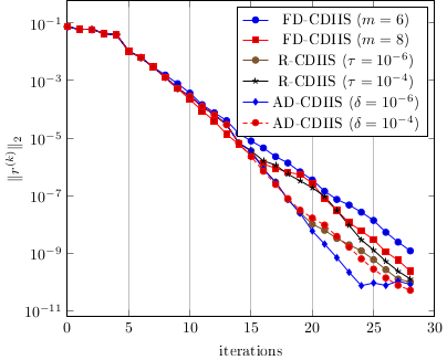
Anderson acceleration, also known as DIIS (Direct Inversion of the Iterative Space) in quantum chemistry, aims to accelerate the convergence of fixed-point iteration $x_{k+1} = g(x_k)$ . Such fixed-point problems are ubiquitous, and in quantum chemistry come from the Hartree-Fock or Kohn-Sham equations. DIIS is an extrapolation method where the next iterate is built using the knowledge of previous iterates. The DIIS sequence is given by

(c^{(k)}_i)_{0 \leq i \leq m} = \argmin_{\sum c_i = 1} \left\|\sum\limits_{i=0}^m c_i f(x_{k-i})\right\|_2 \quad \text{and} \quad x_{k+1} = g\left(\sum_{i=0}^m c^{(k)}_i x_{k-i}\right),

where $f$ is an error function that locally vanishes only at the solution of the fixed-point problem. A usual choice is $f(x) = x-g(x)$ .

An important parameter in the efficiency of the method is the width $m$ of the history/number of iterates kept. Two variants are considered in our publication:

one where the history increases until the least-square problem is ill-conditioned.
another where the size of the history is controlled by the ratio of the residuals $\frac{\|f(x_i)\|}{\|f(x_j)\|}$ for $k-m\leq i,j \leq k$ . The heuristic behind this variant is to keep the iterates that are the most relevant to build the next one.

For both variants, we prove local linear convergence and superlinear convergence by tuning the DIIS numerical parameters.

Comparison between the DIIS variants with fixed depth (FD-DIIS), with restarts (R-DIIS) and adaptive depth (AD-DIIS)

Publication

Maxime Chupin, Mi-Song Dupuy, Guillaume Legendre, Eric Séré, Convergence analysis of adaptive DIIS algorithms with application to electronic ground state calculations, ESIAM: M2AN, (2021).

Solid state physics

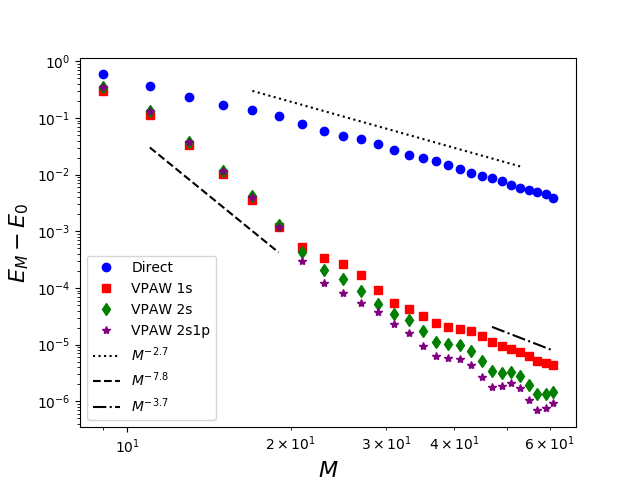
In solid-state physics, the periodic boundary conditions motivate a plane-wave discretisation. However because of the Coulomb singularities at the nuclei, the eigenfunctions of the Hamiltonian $-\Delta + V$ have cusps which impedes the convergence. Pseudopotential methods are widely used, where the Coulomb singularities are smoothened. In the PAW method (Projector Augmented-Wave), introduced by Blöchl, the pseudopotential is introduced using an invertible operator acting locally around the nuclei. The PAW equations involve infinitely many terms that are truncated in the numerical treatment which causes a modelling error. This modelling error has been analysed for the one-dimensional model $-\frac{\mathrm{d}^2}{\mathrm{d}x^2} - Z_0 \sum_{k \in \mathbb{Z}} \delta_k - Z_a\sum_{k \in \mathbb{Z}} \delta_{a+k}$ for which explicit formulas of the eigenpairs are available.

Another approach consists in introducing an invertible operator $T$ acting locally around the nuclei. This operator is defined such that it maps smooth functions to functions with cusps satisfying the Kato cusp condition. This operator acts as a preconditonner for a plane-wave discretisation. This method is called the Variational Projector Augmented-Wave and has been analysed for one-dimensional and three-dimensional Hamiltonians.

Comparison between a direct discretization and the VPAW method for $-\Delta - \frac{1}{|x-R|}-\frac{1}{|x+R|}$ with periodic boundary conditions

Publications

Xavier Blanc, Eric Cancès, Mi-Song Dupuy, Variational projector augmented-wave method : theoretical analysis and preliminary numerical results, Numerische Mathematik, 2019.
Mi-Song Dupuy, Projector augmented-wave method: analysis in a one-dimensional setting, ESAIM: M2AN, 2020.
Mi-Song Dupuy, Variational projector-augmented wave method: a full-potential approach for electronic structure calculations in solid-state physics, Journal of Computational Physics, 2021.