from qat.lang.AQASM import Program
my_program = Program()
qregister = my_program.qalloc(2) #allocates 2 qubits
circuit = my_program.to_circ()
circuit.display()Quantum Computing Notes
Notation
\(\lVert \cdot \rVert\) denotes the Euclidean norm on \(\mathbb{C}^n\). \(^*\) denotes the complex conjugate.
Definition 1 (Kronecker product) For \(A \in \mathbb{C}^{m \times n}\) and \(B \in \mathbb{C}^{p \times q}\), the matrix \(A \otimes B\) is the Kronecker product of \(A\) and \(B\) defined by \[ (A \otimes B)_{ij, k\ell} = A_{ik} B_{j\ell}, \quad \text{for } 1\leq i \leq m, 1 \leq j \leq p, 1 \leq k \leq n, 1 \leq \ell \leq q. \]
Proposition 1 Let \(A,B,C,D\) be matrices of compatible sizes. The following assertions are true
- \((A \otimes B)(C \otimes D) = (AC) \otimes (BD)\)
- \((A \otimes B)^* = A^* \otimes B^*\)
- if \(A\) and \(B\) are unitary matrices, then \(A \otimes B\) is a unitary matrix
- if \((U_A, \Sigma_A, V_A^*)\) and \((U_B, \Sigma_B, V_B^*)\) be singular value decompositions of \(A\) and \(B\), then \((U_A \otimes U_B, \Sigma_A \otimes \Sigma_B, V_A^* \otimes V_B^*)\) is a singular value decomposition of \(A \otimes B\).
The first two statements are consequences of the definition of a Kronecker product. The other statements directly follow from the first two statements.
Basics of Quantum Mechanics
Quantum State
Definition 2 (Quantum state) Let \(N \in \mathbb{N}\). Let \(\sim\) be the equivalence relation on \(\mathbb{C}^N\) defined by \[ \forall\, \phi,\psi \in \mathbb{C}^N, \phi \sim \psi \Leftrightarrow \exists \lambda \not= 0 \in \mathbb{C}, \psi = \lambda \phi. \] Let \(\mathrm{P} \mathbb{C}^N\) be the quotient set \(\mathbb{C}^N\) by \(\sim\). A quantum state is an element of \(\mathrm{P} \mathbb{C}^N\).
Remark 1 (Dirac notation). For \(\psi \in \mathbb{C}^N, \psi \not=0\), the corresponding quantum state is denoted by \(\vert \psi\rangle\). For \(\phi \in (\mathbb{C}^N)^*, \phi \not=0\), the dual quantum state is denoted by \(\langle \phi\vert\). The scalar product between \(\vert \phi\rangle\) and \(\vert \psi\rangle\) is denoted by \(\langle \phi\vert \psi \rangle\). If \(\phi, \psi \in \mathbb{C}^N\) are such that \(\lVert \phi \rVert = \lVert \psi \rVert=1\) then \(\langle \phi\vert \psi \rangle = \sum_{i=1}^N phi_i^* psi_i\).
In the following, we will identify \(\vert \psi\rangle\) to a normalised representing vector \(\psi \in \mathbb{C}^N\). Hence we will write the coordinates of \(\vert \psi\rangle\) in \(\mathbb{C}^N\) as \(\begin{bmatrix} \psi_1 \\ \vdots \\ \psi_N \end{bmatrix}\), where \(\sum_{i=1} |\psi_i|^2 = 1\). Note that by definition of the equivalence class, all vector representations of the form \(\begin{bmatrix} e^{\mathrm{i} \theta}\psi_1 \\ \vdots \\ e^{\mathrm{i} \theta}\psi_N \end{bmatrix}\), for \(\theta \in \mathbb{R}\), are equivalent.
Remark 2. For \(\vert \phi\rangle, \vert \psi\rangle\) quantum states, \(\vert \psi\rangle \langle \phi\vert\) denotes the projection onto \(\psi\) parallel to \(\phi\) and is identified with a matrix \(\mathbb{C}^{N \times N}\).
Evolution of a quantum state
For \(|\psi\rangle\), \(|\phi\rangle\) quantum states, there exists a matrix \(U \in \mathbb{C}^{N \times N}\) such that \(|\psi\rangle = U|\phi\rangle\).
Definition 3 (Schrödinger equation) Let \((H(t))_{t \geq 0}\) be a family of Hermitian matrices, and \(\vert \psi_0\rangle\) a quantum state. The Schrödinger evolution of a quantum state \(t \mapsto \psi(t)\) is defined as the solution to the equation \[ \left\lbrace \begin{aligned} \mathrm{i} \frac{\partial}{\partial t}\psi(t) &= H(t)\psi(t), \quad t \geq 0 \\ \psi(0) &= \psi_0 \end{aligned}\right. \]
One can check that if \(\|\psi_0\|=1\) then for all \(t \geq 0\), \(\|\psi(t)\|=1\).
If \(t \mapsto H(t)\) is constant and equal to \(H\), then the solution to the Schrödinger equation is \(\psi(t) = e^{\mathrm{i} Ht} \psi_0\). This shows that for Hermitian matrices \(H\), the matrix \(e^{\mathrm{i} H}\) is a unitary matrix. Conversely, one can show that any unitary matrix \(U\) can be written as \(e^{\mathrm{i} H}\) for some Hermitian matrix \(H\).
Observables and measurements
Definition 4 (Observable) An observable \(O \in \mathbb{C}^{N \times N}\) is a Hermitian matrix. For \(\vert \psi\rangle\) a quantum state, the expectation value denoted by \(\langle \psi\vert O \vert \psi\rangle\) is equal to \(\langle \psi ,O \psi \rangle\).
Let \(O\) be an observable. Then \(O\) can be written in the basis of its eigenvectors as \(O = \sum_{m=1}^N \lambda_m P_m\), where for \(1 \leq m \leq N\), \(P_m\) orthogonal projector, \(P_m = |u_m\rangle\langle u_m|\). A quantum state \(\vert \psi\rangle\) can be written in the basis \((u_m)\) as \(\psi = \sum_{m=1}^N p_m u_m\), with \(\sum_{m=1}^{N} |p_m|^2 = 1\). Then the expectation value of the observable is \(\langle \psi|O|\psi\rangle = \text{Tr}(|\psi\rangle\langle\psi|O) = \sum_{m=1}^N \lambda_m |p_m|^2\).
Definition 5 (Measurement) Let \(\vert \psi\rangle\) be a quantum state on \(\mathbb{C}^N\) and \(O \in \mathbb{C}^{N \times N}\) be an observable. Let \((u_m)\) be an orthonormal basis of eigenvectors of \(O\). Let \((p_m) \in \mathbb{C}^N\) such that \(\vert \psi\rangle = \sum_{k=1}^{N} p_m u_m\) (with \(\sum_{k=1}^{N} |p_m|^2 = 1\)). The measurement operator \(\mathcal{M}\) for the observable \(O\) is the operator such that \[ \mathcal{M} \vert \psi\rangle = u_m, \quad \text{ with probability } |p_m|^2. \]
The measurement is, for a general quantum state \(\vert \psi\rangle\) and observable \(O\), a nonlinear operator. The output of the measurement is probabilistic and depends on the expansion of the quantum state \(\psi\) in the basis of eigenvectors of the observable \(O\).
Measurements are the only way to have access to the information contained in the quantum state \(\vert \psi\rangle\). For efficient quantum computations, it is thus important that the quantum state obtained after quantum computations has contributions in a few eigenvectors of the measured observable.
Quantum Computer
Qubit
Classical bit: \(b \in \{0, 1\}\)
Definition 6 (Quantum bit (qubit)) A quantum bit (or qubit) is a quantum state on \(\mathbb{C}^2\).
The canonical basis associated to the space of quantum bits on \(\mathbb{C}^2\) is denoted by \(|0\rangle = \begin{bmatrix} 1 \\ 0 \end{bmatrix}\) and \(|1\rangle = \begin{bmatrix} 0 \\ 1 \end{bmatrix}\).
A quantum bit \(|\psi\rangle \in \mathbb{C}^2\) satisfies \(|\psi\rangle = \psi_1|0\rangle + \psi_2|1\rangle\) with \(|\psi_1|^2 + |\psi_2|^2 = 1\) (up to a global phase).
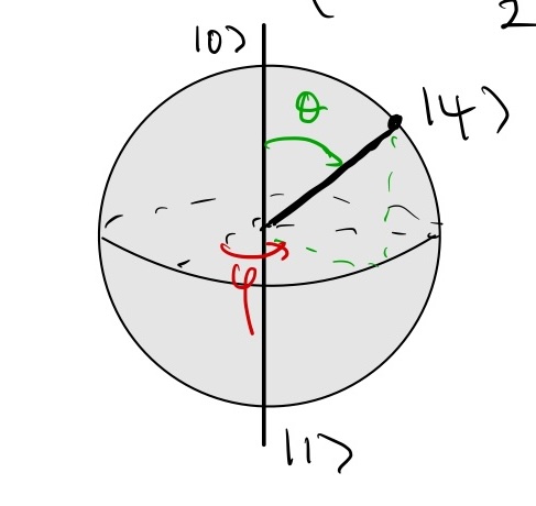
A qubit can be parametrised by two angles Representation on the Bloch sphere: \[ |\psi\rangle = e^{i\gamma}(\cos\frac{\theta}{2}|0\rangle + e^{i\varphi}\sin\frac{\theta}{2}|1\rangle), \] where \(0 \leq \theta \leq \pi\), \(0 \leq \varphi < 2\pi\) (recall that the global phase \(e^{i \gamma}\) is not relevant).
Pauli gates
Definition 7 Let \(X,Y,Z \in \mathbb{C}^{2 \times 2}\) be the Pauli matrices defined by \[ X = \begin{bmatrix} 0 & 1 \\ 1 & 0 \end{bmatrix}, \quad Y = \begin{bmatrix} 0 & -i \\ i & 0 \end{bmatrix}, \quad Z = \begin{bmatrix} 1 & 0 \\ 0 & -1 \end{bmatrix}. \]
Notice that the Pauli matrices \(X,Y,Z\) are Hermitian. They satisfy the commutation relations \([X,Y] = Z, [Y, Z]=X, [Z,X] = Y\). One can show that \((I,X,Y,Z)\) is in fact a basis of Hermitian matrices. This means that unitary evolutions of quantum states can be written as \(e^{\mathrm{i} \theta X + \mathrm{i} \phi Y + \mathrm{i} \gamma Z}\) (as the global phase can be ignored).
This motivates the introduction of parametrised gates \[ e^{ \mathrm{i} \theta/2 X} = \begin{bmatrix} \cos(\theta/2) & -i\sin(\theta/2) \\ -i\sin(\theta/2) & \cos(\theta/2) \end{bmatrix}, \quad e^{ \mathrm{i} \theta/2 Y} =\begin{bmatrix} \cos(\theta/2) & -\sin(\theta/2) \\ \sin(\theta/2) & \cos(\theta/2) \end{bmatrix}, \quad e^{ \mathrm{i} \theta/2 (Z-I)} = \begin{bmatrix} e^{-i\theta/2} & 0 \\ 0 & e^{i\theta/2} \end{bmatrix}. \]
As the matrices \(X,Y,Z\) do not commute, we do not have \(e^{\mathrm{i} \theta X + \mathrm{i} \phi Y + \mathrm{i} \gamma Z} = e^{\mathrm{i} \theta X}e^{\mathrm{i} \phi Y} e^{\mathrm{i} \gamma Z}\). However, using what is called Trotter splitting, we have that \[ e^{\mathrm{i} \theta X + \mathrm{i} \phi Y + \mathrm{i} \gamma Z} = \lim_{n \to \infty} \prod_{i=1}^n e^{\mathrm{i} \theta/n X}e^{\mathrm{i} \phi/n Y} e^{\mathrm{i} \gamma/n Z}, \] which motivates the use of the parametrised gates introduced above.
Measurement of one qubit
Measurements of a qubit are taken for the observable \(Z\) (except otherwise stated). The computational basis \(\vert 0\rangle, \vert 1\rangle\) is the basis that diagonalises \(Z\), thus the measurement of a quantum state \(| \psi \rangle = \psi_0 | 0 \rangle + \psi_1 |1 \rangle,\) gives \(\vert 0\rangle\) with probability \(p_0 = |\psi_0|^2\) and \(\vert 1\rangle\) with probability \(p_1 = |\psi_1|^2 = 1-p_0\).
This means that the measurement is a Bernoulli random variable. The variance related to the estimation of the probability \(p_0\) is equal to \(p_0(1 - p_0)\).
To estimate \(p_0\), one uses the empirical estimator \(\hat{p}_0 = \frac{\text{number of measured } |0\rangle}{\text{total number of samples}}\). If \(\mathcal{N}\) is the total number of samples, and assuming that each measurement is independent, the variance of the empirical estimator is \(\frac{p_0(1-p_0)}{\mathcal{N}}\). To guarantee that the standard deviation of the empirical estimator is below some threshold \(\epsilon\), we must have \(\frac{p_0(1-p_0)}{\mathcal{N}} \leq \epsilon^2\), thus \(\mathcal{N} \geq \frac{p_0(1-p_0)}{\epsilon^2}\).
For a small probability \(p_0\), an accurate estimation of the probability \(p_0\) requires to have \(\epsilon \ll p_0\), which means that the number of samples needs to be much larger than \(\frac{1}{p_0}\). This is another important restriction in designing efficient algorithms in quantum computing.
Other important one-qubit gates
| Function | Description | Matrix Representation | Usage |
|---|---|---|---|
| H | Hadamard gate | \(\begin{bmatrix} \frac{1}{\sqrt{2}} & \frac{1}{\sqrt{2}} \\ \frac{1}{\sqrt{2}} & -\frac{1}{\sqrt{2}} \end{bmatrix}\) | H(qubit) |
| S | Phase gate (or S gate) | \(\begin{bmatrix} 1 & 0 \\ 0 & i \end{bmatrix}\) | S(qubit) |
| T | T gate | \(\begin{bmatrix} 1 & 0 \\ 0 & e^{i\pi/4} \end{bmatrix}\) | T(qubit) |
Collection of many qubits or the quantum register
A classical register is a collection of classical bits \(b = (b_1, \ldots, b_n)\), \(b_i \in \{0, 1\}\), \(i = 1, \ldots, n\).
Definition 8 (Quantum register) A quantum register on \(n\) qubits is a quantum state on \(\bigotimes_{i=1}^n \mathbb{C}^{2}\).
The space \(\bigotimes_{i=1}^n \mathbb{C}^{2}\) can be identified with \(\mathbb{C}^{2^n}\). Its canonical basis, also called the computational basis is the set of the canonical basis of \(\mathbb{C}^{2^n}\). These vectors are denoted by \(\vert q_1 \dots q_n\rangle\), where \((q_k) \in \lbrace 0,1 \rbrace\). They correspond to the \(j-th\) canonical vector, \(j \in \lbrace 0, \dots, 2^n-1 \rbrace\), where \(j = \sum_{k=1}^{n} q_k 2^{-k}\) (i.e. \((q_k)\) is the binary decomposition of \(j\)). It is also customary to denote the quantum state \(\vert j\rangle\).
Example 1 (Kronecker products of qubits) If \(|\psi_1\rangle \in \mathbb{C}^2\), \(|\psi_2\rangle \in \mathbb{C}^2\), \(|\psi\rangle = |\psi_1\rangle \otimes |\psi_2\rangle\) is a 2-qubit state.
\(|0\rangle \otimes |0\rangle = \begin{bmatrix} 1 \\ 0 \end{bmatrix} \otimes \begin{bmatrix} 1 \\ 0 \end{bmatrix} = \begin{bmatrix} 1 \\ 0 \\ 0 \\ 0 \end{bmatrix}\)
Remark 3 (Entanglement). The quantum states seen so far are given as Kronecker products. The power of quantum computing lies in the manipulation of entangled states, that cannot be obtained from Kronecker products of quantum states. For example, the Bell state \(|\psi\rangle = \frac{1}{\sqrt{2}}(|0\rangle \otimes |0\rangle + |1\rangle \otimes |1\rangle)\) cannot be written as a Kronecker product of one qubit state.
No-Cloning Theorem
Theorem 1 (No cloning) Let \(\vert s \rangle \in \mathbb{C}^n\) be a quantum state. There is no unitary matrix \(U \in \mathbb{C}^{n^2 \times n^2}\) such that for any \(\vert \psi\rangle \in \mathbb{C}^n\), we have
\[
U |\psi \rangle \otimes | s \rangle = |\psi \rangle \otimes | \psi \rangle.
\]
Proof. Let \(U\) be such that for any \(\vert \psi\rangle \in \mathbb{C}^n\), we have
\[
U |\psi \rangle \otimes | s \rangle = |\psi \rangle \otimes | \psi \rangle.
\] Let \(\vert \phi\rangle \in \mathbb{C}^n\) such that \(\langle \phi \vert \psi \rangle \not= 0\) or 1. Then \(U \vert \phi\rangle \otimes \vert s \rangle = \vert \phi\rangle \otimes \vert \phi\rangle\). Thus we have \[
\begin{aligned}
\langle \phi | \otimes \langle \phi | \psi \rangle \otimes | \psi \rangle &= \langle s | \otimes \langle \phi | U^* U | s \rangle \otimes | \psi \rangle \\
\langle \phi | \psi \rangle^2 &= \langle \phi | \psi \rangle.
\end{aligned}
\] This means that either \(\langle \phi | \psi \rangle = 0\) or \(\langle \phi | \psi \rangle = 1\): contradiction.
This theorem has a crucial consequence in the design of quantum algorithms: a vast majority of classical algorithms are iterative (Newton, root finding, conjugate-gradient…) which requires to store a copy of some iterate. In quantum computing, as it is impossible to copy arbitrary quantum states, the design of quantum algorithms cannot be a simple transposition of efficient classical algorithms.
Following the proof of the no-cloning theorem, it is however possible to copy some quantum states:
- for known quantum states \(\vert \psi\rangle\), \(\vert s \rangle\), if a unitary \(U_\psi\) such that \(U_\psi \vert s\rangle = \vert \psi\rangle\), then \((I \otimes U_\psi)(| \psi \rangle \otimes | s \rangle) = | \psi \rangle \otimes | \psi \rangle\);
- for quantum state \(\vert j\rangle\) in the computational basis, then any state \(\vert k \rangle\) in the computational basis can be copied, i.e. for any \(0 \leq j \leq n-1\), there is \(U\) such that for any \(0 \leq k \leq n-1\), we have \[ U | k \rangle \otimes | j \rangle = | k \rangle \otimes | k \rangle. \] For \(n=4\) and \(j=0\), this unitary is the \(\mathrm{CNOT}\) gate: \(\mathrm{CNOT}(| k \rangle \otimes | 0 \rangle) = | k \rangle \otimes | k \rangle\). One can check that if \(\vert \psi \rangle = \psi_0 \vert 0\rangle + \psi_1 \vert 1\rangle\) with \(\psi_0 \psi_1 \not=0\), then \(\mathrm{CNOT} \vert \psi\rangle \otimes \vert 0\rangle = \psi_0 \vert 00\rangle + \psi_1 \vert 11\rangle \not= \vert \psi\rangle \otimes \vert \psi\rangle\).
Gates
Linear operations on quantum registers are called gates. These linear operations are necessarily unitary operators.
In classical computing, any operation on classical registers can be implemented using combinations of only a few gates (for example, using only NAND or NOR gates).
In quantum computing, any operation can be implemented using only one or two-qubit gates (i.e. gates that operate only on one or two qubits).
It is possible to further restrict this set, if we give up on the exact representation of the unitary \(U\), i.e. for a given accuracy \(\epsilon>0\), we want to find \((U_1,\dots,U_m)\) such that
- \(\lVert U - U_m U_{m-1} \cdots U_1 \rVert < \epsilon\),
- \((U_k)_{1\leq k \leq m}\) belongs to a (small) set of universal gates.
There are multiple choices of universal gates such as \(\lbrace H, T, \mathrm{CNOT} \rbrace\) or \(\lbrace H, \mathrm{Toffoli} \rbrace\) (see their definitions below). A natural question is to check whether there are sets of universal gates that are better than others. The answer is given by the following theorem.
Theorem 2 (Solovay-Kitaev) Let \(\mathcal{S}, \mathcal{T}\) be two sets of universal gates that are closed under inverses. Then any \(m\)-gate circuit using the gate set \(\mathcal{S}\) can be implemented to precision \(\epsilon\) using a circuit of \(\mathcal{O}(m \, \mathrm{polylog}(m/ϵ))\) gates from the gate set \(\mathcal{T}\).
Asymptotically, the Solovay-Kitaev theorem states that any choice of sets of universal gates leads to a comparable number of quantum operations.
Summary of the common quantum gates
Here is a list of common quantum gates as well as the corresponding command in MyQLM. A quantum algorithm is simply a series of quantum gates applied to a initial quantum state (which is generally the state \(\vert 0 \rangle\)).
Constant gates
| Function | Description | Matrix Representation | Usage |
|---|---|---|---|
| X | Pauli-X gate, NOT gate | \(\begin{bmatrix} 0 & 1 \\ 1 & 0 \end{bmatrix}\) | X(qubit) |
| Y | Pauli-Y gate | \(\begin{bmatrix} 0 & -i \\ i & 0 \end{bmatrix}\) | Y(qubit) |
| Z | Pauli-Z gate | \(\begin{bmatrix} 1 & 0 \\ 0 & -1 \end{bmatrix}\) | Z(qubit) |
| H | Hadamard gate | \(\begin{bmatrix} \frac{1}{\sqrt{2}} & \frac{1}{\sqrt{2}} \\ \frac{1}{\sqrt{2}} & -\frac{1}{\sqrt{2}} \end{bmatrix}\) | H(qubit) |
| S | Phase gate (or S gate) | \(\begin{bmatrix} 1 & 0 \\ 0 & i \end{bmatrix}\) | S(qubit) |
| T | T gate | \(\begin{bmatrix} 1 & 0 \\ 0 & e^{i\pi/4} \end{bmatrix}\) | T(qubit) |
| CNOT | CNOT (Controlled NOT) gate | \(\begin{bmatrix} 1 & 0 & 0 & 0 \\ 0 & 1 & 0 & 0 \\ 0 & 0 & 0 & 1 \\ 0 & 0 & 1 & 0 \end{bmatrix}\) | CNOT(control_qubit, target_qubit) |
| CCNOT | Toffoli gate (or CCNOT gate). | \(\begin{bmatrix} 1 & 0 & 0 & 0 & 0 & 0 & 0 & 0 \\ 0 & 1 & 0 & 0 & 0 & 0 & 0 & 0 \\ 0 & 0 & 1 & 0 & 0 & 0 & 0 & 0 \\ 0 & 0 & 0 & 1 & 0 & 0 & 0 & 0 \\ 0 & 0 & 0 & 0 & 1 & 0 & 0 & 0 \\ 0 & 0 & 0 & 0 & 0 & 1 & 0 & 0 \\ 0 & 0 & 0 & 0 & 0 & 0 & 0 & 1 \\ 0 & 0 & 0 & 0 & 0 & 0 & 1 & 0 \end{bmatrix}\) | CCNOT(control_qubit1, control_qubit2, target_qubit) |
| CSIGN | Controlled Sign or C-Z gate | \(\begin{bmatrix} 1 & 0 & 0 & 0 \\ 0 & 1 & 0 & 0 \\ 0 & 0 & 1 & 0 \\ 0 & 0 & 0 & -1 \end{bmatrix}\) | CSIGN(control_qubit, target_qubit) |
| SWAP | SWAP gate | \(\begin{bmatrix} 1 & 0 & 0 & 0 \\ 0 & 0 & 1 & 0 \\ 0 & 1 & 0 & 0 \\ 0 & 0 & 0 & 1 \end{bmatrix}\) | SWAP(qubit1, qubit2) |
| SQRTSWAP | Square Root of SWAP gate. It creates a superposition of swapped and non-swapped states. | \(\begin{bmatrix} 1 & 0 & 0 & 0 \\ 0 & \frac{1}{2}(1+i) & \frac{1}{2}(1-i) & 0 \\ 0 & \frac{1}{2}(1-i) & \frac{1}{2}(1+i) & 0 \\ 0 & 0 & 0 & 1 \end{bmatrix}\) | SQRTSWAP(qubit1, qubit2) |
| ISWAP | iSWAP gate. It swaps the states of two qubits with a phase factor of i. | \(\begin{bmatrix} 1 & 0 & 0 & 0 \\ 0 & 0 & i & 0 \\ 0 & i & 0 & 0 \\ 0 & 0 & 0 & 1 \end{bmatrix}\) | ISWAP(qubit1, qubit2) |
In this list, the \(\mathrm{CNOT},\mathrm{CSIGN}, \mathrm{SWAP}, \mathrm{SQRTSWAP}\) and \(\mathrm{ISWAP}\) are unitary operators acting on two qubits. It can be proved that these unitary operations cannot be written as the Kronecker product of two one-qubit gates.
The \(\mathrm{Toffoli}\) gate is a 3-qubit gate that also cannot be written as a Kronecker product of one-qubit gates.
Parametrised gates
| Function | Description | Matrix Representation | Usage |
|---|---|---|---|
| RX(θ) | Rotation around the X-axis by an angle θ. | \(\begin{bmatrix} \cos(\theta/2) & -i\sin(\theta/2) \\ -i\sin(\theta/2) & \cos(\theta/2) \end{bmatrix}\) | RX(theta)(qubit) |
| RY(θ) | Rotation around the Y-axis by an angle θ. | \(\begin{bmatrix} \cos(\theta/2) & -\sin(\theta/2) \\ \sin(\theta/2) & \cos(\theta/2) \end{bmatrix}\) | RY(theta)(qubit) |
| RZ(θ) | Rotation around the Z-axis by an angle θ. | \(\begin{bmatrix} e^{-i\theta/2} & 0 \\ 0 & e^{i\theta/2} \end{bmatrix}\) | RZ(theta)(qubit) |
| PH(φ) | Phase gate that leaves \(\vert 0\rangle\) unchanged and maps \(\vert 1\rangle\) to \(e^{iφ}\vert 1\rangle\). | \(\begin{bmatrix} 1 & 0 \\ 0 & e^{iφ} \end{bmatrix}\) | PH(phi)(qubit) |
Quantum circuit
Quantum circuits are graphical representations of quantum algorithms. They show how quantum gates are applied to qubits over time.
Qubits and Wires
- Qubits: each qubit is represented by one horizontal line (a wire) in a circuit diagram.
- Initial State: qubits start in the \(\vert 0\rangle\) state unless otherwise specified.
Example in MyQLM
The following piece of code displays a quantum register initialised (by default) at \(\vert 00\rangle\).
Gates
Gates are represented by boxes or dots in the quantum circuit. Their applications are read from left to right.
Example for one qubit in MyQLM
The following piece of code displays the quantum algorithm \(X H \vert 0\rangle\).
from qat.lang.AQASM import Program
from qat.lang.AQASM import H, X #import the Hadamard gate and the CNOT gate
my_program = Program()
qregister = my_program.qalloc(1) #allocates 2 qubits
H(qregister[0]) #first apply Hadamard gate
X(qregister[0]) #then apply X gate
circuit = my_program.to_circ()
circuit.display()Example for two qubits in MyQLM
The following piece of code displays the quantum algorithm \((I \otimes Y) (X \otimes I) (H \otimes I) \vert 0 0\rangle\).
from qat.lang.AQASM import Program
from qat.lang.AQASM import H, X, Y #import the Hadamard gate and the CNOT gate
my_program = Program()
qregister = my_program.qalloc(2) #allocates 2 qubits
H(qregister[0]) #first apply Hadamard gate on the first qubit
X(qregister[0]) #then apply X gate on the first qubit
Y(qregister[1]) #then apply X gate on the first qubit
circuit = my_program.to_circ()
circuit.display()Note that since \((I \otimes Y)\) and \((X \otimes I) (H \otimes I)\), the quantum operations are squashed to the left.
CNOT gate in MyQLM
The following piece of code displays the quantum algorithm \(\mathrm{CNOT} \vert 0 0\rangle\).
from qat.lang.AQASM import Program
from qat.lang.AQASM import CNOT #import the Hadamard gate and the CNOT gate
my_program = Program()
qregister = my_program.qalloc(2) #allocates 2 qubits
CNOT(qregister[0],qregister[1]) #first apply the CNOT gate with the 1st qubit as the control and 2nd as the target
circuit = my_program.to_circ()
circuit.display()SWAP gate in MyQLM
The following piece of code displays the quantum algorithm \(\mathrm{SWAP} \vert 0 0\rangle\).
from qat.lang.AQASM import Program
from qat.lang.AQASM import SWAP #import the Hadamard gate and the CNOT gate
my_program = Program()
qregister = my_program.qalloc(2) #allocates 2 qubits
SWAP(qregister[0],qregister[1]) #first apply the CNOT gate with the 1st qubit as the control and 2nd as the target
circuit = my_program.to_circ()
circuit.display()Complexity of a quantum algorithm
Remark 4 (Clifford gates). Clifford gates are quantum gates that stabilises the group formed by Kronecker products of Pauli matrices (i.e. if \(C\) is a Clifford gate and \(P\) a Kronecker product of Pauli matrices, then \(C P C^*\) is a Kronecker product of Pauli matrices). It can be checked that the Hadamard gate, the CNOT gate are Clifford gates, but not the \(T\) gate. Since these gates stabilise the group of Kronecker product of Pauli matrices, they can be classically simulated in polynomial time.
The complexity of quantum algorithms is estimated in three different ways:
- the depth of the circuit: the depth of the circuit is the maximal number of gates along any path from an input and an output. It is a reasonable depiction of the total run time of a quantum simulation. One of the main challenge in the design of physical quantum computers is in maintaining the coherence time of the quantum system. The coherence time is the longest period during which the quantum system accurately preserves the outcome of a quantum algorithm. Nowadays, the maximal coherence time is of the order of \(0.1\) ms and the total number of operations that can be performed is of the order \(10^2, 10^3\).
- the number of two qubit gates in the quantum algorithm: \(\mathrm{CNOT}\) gates have a probability of failure of about 1%, whereas one-qubit gates typically have failure rates of about \(0.1\)% (or sometimes lower than that). The accuracy of a quantum algorithm depends heavily on the number of two-qubit gates.
- the number of \(T\) gates in the quantum algorithm: to a lesser extend, the complexity of a quantum algorithm can also be estimated by counting the number of \(T\) gates. If a quantum algorithm is expressed in the universal gate set \(\lbrace H, T, \mathrm{CNOT} \rbrace\), the only non-Clifford gate is the \(T\) gate. As Clifford gates are classically easy to emulate, the quantum advantage can be estimated as the total number of \(T\) gates.